Supplementary Data
Thermal explosion: when is a solid-state
self-sustained reaction front formed?
The
Frank-Kamenetskii criterion revisited.
D. Sánchez-Rodriguez,
J. Farjas*, P. Roura.
University of Girona, Campus Montilivi, Edif. PII, E17071 Girona, Catalonia, Spain
An implicit finite differences scheme has been
used to numerically solve the 1D model, while an alternating-direction
semi-implicit finite differences method has been used for the 2D case [1]. In the following sections we describe the
numerical approach used to solve the following set of equations:
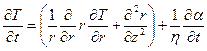 (S1)
(S1)
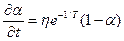 (S2)
(S2)
 (S3)
(S3)
The system of Eqs.
S1-S3 is dimensionless, i.e., in the following all variables are dimensionless.
First we describe the 1D models that arises when we neglect one term of the laplacian. Afterwards we describe the integration of the
reaction kinetics. Next we address the presence of an interface between the
sample and a substrate and finally we describe the 2D model. Finally we provide
some relevant details on the use of the program.
1. 1D
model without substrate: implicit scheme.
First we will consider the case
 , so we can neglect the partial derivative with respect r. The finite
differences method is based on the discretization of space and time [1]:
, so we can neglect the partial derivative with respect r. The finite
differences method is based on the discretization of space and time [1]:
 , (S4)
where  is the grid spacing
and
is the grid spacing
and  is the time step used
in the discretization. Under the explicit scheme, Eq. S1 becomes:
is the time step used
in the discretization. Under the explicit scheme, Eq. S1 becomes:
 (S5)
(S5)
where  ,
,  ,
,  and N is the number of points of the space
grid. At a given time tn
and from the temperatures of the previous iteration and knowing
and N is the number of points of the space
grid. At a given time tn
and from the temperatures of the previous iteration and knowing
 , it is straightforward to calculate
  from Eq. S5. However,
the stability criterion of the explicit scheme imposes that
from Eq. S5. However,
the stability criterion of the explicit scheme imposes that  . This criterion represent a very restrictive constraint for
the time step . Since Eqs.
S1 and S3 involve very different time scales; this constraint represents a
drastic limitation on the parameter range that can be explored numerically.
Thus, the use of an implicit integration method is
mandatory. Under the implicit scheme Eq. S1 becomes:
. This criterion represent a very restrictive constraint for
the time step . Since Eqs.
S1 and S3 involve very different time scales; this constraint represents a
drastic limitation on the parameter range that can be explored numerically.
Thus, the use of an implicit integration method is
mandatory. Under the implicit scheme Eq. S1 becomes:
 (S6)
(S6)
In Eq. S6 we have 4 unknowns, namely
,  ,
,  and , therefore, unlike the explicit method, the temperatures at
time tn
cannot be directly determined from the differential equation. However, if we
ignore the dependence of on , Eq. 6 is a tridiagonal system
that can be solved:
and , therefore, unlike the explicit method, the temperatures at
time tn
cannot be directly determined from the differential equation. However, if we
ignore the dependence of on , Eq. 6 is a tridiagonal system
that can be solved:
 (S7)
(S7)
Thus, once we know ,
,  and
and  the values of can be directly
calculated from Eq. S7. is
determined from the boundary conditions; from Eq. S3
the values of can be directly
calculated from Eq. S7. is
determined from the boundary conditions; from Eq. S3  . As for the coefficients and , substitution of Eq. S7 in Eq. S6 gives,
 (S8)
(S8)
where  and the coefficients
  and
and  are determined from
the boundary conditions; from Eqs. S3 and S7 one
obtains
are determined from
the boundary conditions; from Eqs. S3 and S7 one
obtains  and
and  . Note, that for the explicit scheme, the stability criterion
imposes
. Note, that for the explicit scheme, the stability criterion
imposes  . Thanks to the use of the implicit scheme we have been able
to use a value of
. Thanks to the use of the implicit scheme we have been able
to use a value of  . Needless to say that no computer in earth
may be able to do the same calculation but using and explicit scheme.
. Needless to say that no computer in earth
may be able to do the same calculation but using and explicit scheme.
However, depends on (in the next section
we describe the calculation of from Eq. S2),
therefore nor the explicit neither the implicit scheme may be directly applied.
We overcome this problem through an iterative procedure. First is calculate assuming that  , then the values of are calculated using
Eq. S7. From the new values of we can determine and again the new
values of . We repeat the iterative procedure until the relative error
in the determination of is below a certain value.
Typically this value is one or two orders of magnitude the smallest
representable floating-point number, e.g., 10-14 to 10-15.
, then the values of are calculated using
Eq. S7. From the new values of we can determine and again the new
values of . We repeat the iterative procedure until the relative error
in the determination of is below a certain value.
Typically this value is one or two orders of magnitude the smallest
representable floating-point number, e.g., 10-14 to 10-15.
For the case  , we can neglect the partial derivative with respect z and
under the implicit scheme, Eq. S1 becomes:
, we can neglect the partial derivative with respect z and
under the implicit scheme, Eq. S1 becomes:
 (S9)
(S9)
And the coefficients and become for the radial
integration,
 (S10)
(S10)
2. Integration of the
reaction kinetics
At a given iteration, the value of is given by Eq. S2.
Eq. S2 may be solved by finite differences, but since the time scale of the
reaction may be significantly smaller than that of diffusion, is very important
to determine as accurately as possible
to improve the stability of the calculus. So instead of solving Eq. S2 by
finite differences, we integrate analytically S2; for [2],
 (S11)
(S11)
where 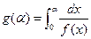 ,
,  and G(z)
is the inverse function of g(α). The expression of G and g for a number of reaction models is given in Ref. [3]. For
instance, for a first order reaction;
and G(z)
is the inverse function of g(α). The expression of G and g for a number of reaction models is given in Ref. [3]. For
instance, for a first order reaction;  ,
,  ,
,  and
and  .
.
For
 , we perform a linear interpolation, i.e., we assume that the
temperature increases linearly between
, we perform a linear interpolation, i.e., we assume that the
temperature increases linearly between  and during the time
interval . The integration of S2 gives [2],
and during the time
interval . The integration of S2 gives [2],
 (S12)
(S12)
where,  and
and 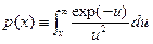 . p(x) has no analytical solution. Since the
integration of p(x) would be very time consuming, we use the Padé
expansion given in Ref. [2] that
is accurate enough for double precision calculations.
. p(x) has no analytical solution. Since the
integration of p(x) would be very time consuming, we use the Padé
expansion given in Ref. [2] that
is accurate enough for double precision calculations.
3. 1D interface
In this section we analyze the effect of an interface between sample and substrate where thermal parameters change. In the interface we impose the continuity of heat flow, but also, the element of the grid at the interface has a certain volume. Half of this volume belongs to the sample, so heat is generated due to the reaction; also the heat capacity is different at both sides of the interface. Therefore at the interface the finite differences equation is,
 (S13)
(S13)
And the coefficients  and
and  become,
 (S14)
(S14)
where I stands for the index of the element of
the grid that is located at the interface, λ
and λs
are the sample and substrate conductivities respectively, 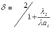 , and as is the substrate
diffusivity (note that the dimensionless diffusivity of the sample is 1).
, and as is the substrate
diffusivity (note that the dimensionless diffusivity of the sample is 1).
4. 2D Integration. Alternating-direction semi-implicit
finite differences method.
Contrarily
to the 1D case, the 2D diffusion equation cannot be solved analytically [1]. This problem can be solved with the alternating-direction
implicit method [1]. This approach consists in splitting the
integration in two time steps  where one of the
directions is calculated implicitly and the other explicitly. We have chosen to
first calculate the radial coordinate implicitly and afterwards the axial
coordinate implicitly. For the first step the finite differences equation is,
where one of the
directions is calculated implicitly and the other explicitly. We have chosen to
first calculate the radial coordinate implicitly and afterwards the axial
coordinate implicitly. For the first step the finite differences equation is,
 (S.15)
where  ,
, 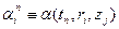 ,
,  ,
,  , and Nr
and Nz
are the number of points of the radial and axial grids respectively.
, and Nr
and Nz
are the number of points of the radial and axial grids respectively.
And the coefficients and become for the radial
implicit integration,
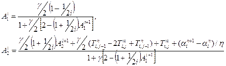 (S16)
(S16)
For the second step the finite differences equation is,
 . (S.17)
And the coefficients and become for the axial
implicit integration,
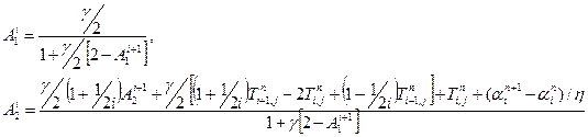 (S16)
(S16)
5. Specifications
Three different programs are included that correspond to (named 1D_cart), (named 1D_radial) and
the 2D case (2D_cil). The data is introduced trough and ascii file, an example of each program is included.
The data is passed to the exe file by sliding the data file into the exe file.
All programs generate a file named “Avg_alpha.dat” that contains the time evolution of the reaction, a set of files named "FrontXXX.dat" that contain the temperature and α profiles at selected times, and a file named "PropFont.dat" that contains the evolution of the position and width of the combustion front. In addition, the 2D program generates a series of images (in format bitmap, bmp) that contain the temperature and α values as a function of coordinates r and z at selected times. This images may be joined to form the movies includes in this paper. To create the movies we have used the freeware EasyBMPtoAVI program [4].
The program has been written in C++. The source files can be directly compiled with Visual Studio 2008. However, the code can be very easily adapted to be compiled in other platforms.
The
following sources have been included:
Download
code for 1D Cartesian
Download code for 2D cylindrical
References
[1] W.H.
Press, B.P. Flannery, S.A. Teukolsky, W.T. Vetterling, Numerical recipes in C: the art of scientific
computing, Cambridge University Press, Cambridge, 1994.
[2] J.
Farjas, P. Roura, Isoconversional analysis of solid state transformations. A critical review. Part I. Single step
transformations with constant activation energy, J. Therm. Anal. Calorim.
105 (2011) 757–766. doi:10.1007/s10973-011-1446-4.
[3] J.
Farjas, P. Roura, Simple
approximate analytical solution for nonisothermal
single-step transformations: Kinetic analysis, AIChE
J. 54 (2008) 2145–2154. doi:10.1002/aic.11540.
[4] http://easybmptoavi.sourceforge.net/,
last access on the 14th july
2014.